1. Filter of Original Signal
In order to filter out the low-frequency content of the original signal (low-key chord of the piano music) which can sometimes be abnormally strong, we apply a high-pass filter to the signal. For some cases, we might be interested in detecting the low-key chord of the music. But for this project, we will only focus on tracking the major melody of the music. The cutoff frequency of the filter is set to be about 200Hz, which corresponds to G3. The filter is designed with the Matlab filter design tool.
Figure 1 below shows the DFT magnitude of a small piece of music. Figure 2 shows the DFT magnitude of the filtered signal.

Figure 1. Music Signal before Filtering

Figure 2. Music Signal After Filtering
2. Pitch-Detection Methods
The visualization of the music is mainly based on the pitch-detections results. A good visualization requires extremely robust pitch-detection algorithms; so we tried three different detection methods, which are FFT method, Cepstral analysis method, and autocorrelation method.
-
FFT Method
The FFT method is the most basic method for pitch detection. We first window the music signal into groups of samples, and then apply the length-N DFT to the windowed signal.

Then the pitch can be determined by finding the peak of the DFT. When determining the DFT length N, we have to trade off between time resolution and frequency resolution. We chose a value between 1000-2000 so that resolutions in both domains are satisfying. This method presents high accuracy for single-pitch detection (only one piano note presents at the same time). However, frequent octave errors and outliers can make the visualization methods fail.
-
Cepstral Analysis Method
Cepstral analysis is a very popular method for speech recognition. In order to find the pitch of the music signal, we first window the signal with Hamming window, and then take the length-N DFT of the windowed signal. Again we have to trade off between time resolution and frequency reolution. Then we take the logarithm of the frequency spectrum. Finally, the pitch can be found by examining the inverse DTFT in a limited range. We implemented this method in Matlab, but this method doesn’t seem to work well for piano notes detection.
-
Autocorrelation Method
The autocorrelation method is based on the autocorrelation function, which measures the extent to which a signal correlates with a delayed version of itself:
For periodic signals like sinusoidal signal, the signal would correlate strongly with itself when delayed by its fundamental period. Therefore, by examining the magnitude and finding the peak of the autocorrelation function, we can roughly find the fundamental period of the signal. The pitch can then be determined from the fundamental period and the sampling frequency. This method presents great robustness and detection accuracy. However, it performs poorly when the music tempo becomes fast. Figure 3 below thows the detection results of the autocorrelation method for a small piece of piano music.


Figure 3. Detection Results of Autocorrelation Method
3. Filter of Detection Results
As mentioned in the previous section, the visualization method of this project requires great robustness of the detection algorithms. However, there can always be some outliers in the detection results.
Different from some other projects, a challenge of this project is that we are doing pitch-detection for a long piece of music, and piano notes are played consecutively. This makes it worse concerning outliers in the detection results.
The goal of this step is to remove the outliers of the detection results. The method we use here is passing the detection results through a moving-median filter. The filter can be described by the equation below, where F is the sequence containing the pitch-detection results:
The following figure shows the filtered detection results. We can see that some of the outliers are removed; however, some are still there. This means that our detection results are always non-ideal. And this becomes one of our main considerations when implementing the visualization methods.
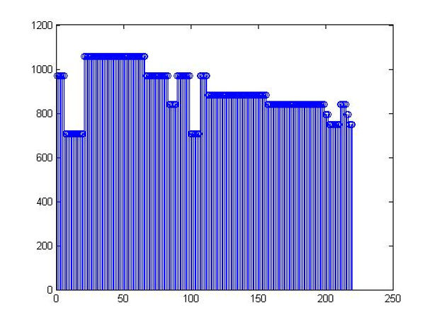
Figure 4. Filtered Pitch-detection Results
4. Visualization Methods
The visualization is based on the pitch and dB magnitude of the music. In order to intuitively visualize these two audio features, we developed two different methods. Both of the two visualizations are synchronous with the audio. These two methods can also be combined into a single visualization window to give better results.
-
Method 1
The first visualization method is to draw a trajectory in the 2D space, where the x-axis represents time and y-axis represents the pitch of the music. We then make a round circle move on the trajectory. Because the scales of the time-axis and the frequency axis are different, we actually have to draw elliptical shapes instead of circle. The position of the circle indicates which key is being played. The Matlab "fill" command is used to make the round circle colorful.
-
Method 2
The second visualization method is also implemented in the 2D space. For this method, the fixed x-axis represents different pitches. Whenever a new piano note comes, we generate a pulse at the point corresponding to that particular pitch. In order to make the pulse natural and smooth, we model the instantaneous height of the pulse by the following equation:

This equation is just the one that models the trajectory of a ball thrown vertically up with initial velocity v0. The initial velocity v0 in our visualization is determined by the dB magnitude at the time when the new note comes. In order to make the visualization look better, we also assign each pitch a unique color so that different pulses are of different colors.
A screenshot of the visualization is shown below. Please see the "Demo" section for a video demo of our project.

Figure 5. screenshot of the visualization